The goal of this project is to make a controller which lands a rocket at a landing pad with at the end of a given time frame. The rockets will start in random initial states and will be subjected to gravity and drag. The rocket will control its angle and thrust.
The current state, X, of the rocket is made of the location of the rocket in relation to the target landing site (d_x and d_y), the current velocity of the rocket (v_x and v_y), and the rocket's angle (theta).
The input, a, of the rocket consists of the acceleration,
The model of drag used in this problem is vastly simplified and will be soley a function of the airspeed, the air desity and a constant, where
Additionally, the coefficient of drag is arbitrarily set to give a predermined terminal velocity at sea level with:
at
We will use a contoller
Where W is a vector containing the weights of each state.
Therefore, the objective is:
In the code below e was calculated as:
e = sum(W[0] * state[:, 0] ** 2 + W[1] * state[:, 1] ** 2 + W[2] * (state[:, 2] - PLATFORM_HEIGHT) ** 2 + W[3] * state[:, 3] ** 2)
# overhead
import logging
# import math
import random
import numpy as np
# import time
import torch as t
import torch.nn as nn
from torch import optim
# from torch.nn import utils
import matplotlib.pyplot as plt
logger = logging.getLogger(__name__)
# environment parameters
FRAME_TIME = 0.1 # time interval
GRAVITY_ACCEL = 0.12 # gravity constant
BOOST_ACCEL = 0.4 # thrust constant
PLATFORM_WIDTH = 0.25 # landing platform width
PLATFORM_HEIGHT = 0.6 # landing platform height
ROTATION_ACCEL = 10 # rotation constant
airDensitySeaLevel = .012250
terminalVel = 1000 # terminal velocity at sea level
C_d = GRAVITY_ACCEL / (airDensitySeaLevel * terminalVel ** 2)
airDensityConstant = -1.186 * 10 ** -6
W = [11, 2., 11., 3.]
numTestStates = 1000
numOfEpochs = 100
# define system dynamics
# Notes:
# 0. You only need to modify the "forward" function
# 1. All variables in "forward" need to be PyTorch tensors.
# 2. All math operations in "forward" has to be differentiable, e.g., default PyTorch functions.
# 3. Do not use inplace operations, e.g., x += 1. Please see the following section for an example that does not work.
class Dynamics(nn.Module):
def __init__(self):
super(Dynamics, self).__init__()
@staticmethod
def forward(state, action):
"""
action[0] = thrust controller
action[1] = omega controller
state[0] = x
state[1] = x_dot
state[2] = y
state[3] = y_dot
state[4] = theta
"""
# Apply gravity
# Note: Here gravity is used to change velocity which is the second element of the state vector
# Normally, we would do x[1] = x[1] + gravity * delta_time
# but this is not allowed in PyTorch since it overwrites one variable (x[1]) that is part of the computational graph to be differentiated.
# Therefore, I define a tensor dx = [0., gravity * delta_time], and do x = x + dx. This is allowed...
delta_state_gravity = t.tensor([0., 0., 0., -GRAVITY_ACCEL * FRAME_TIME, 0.])
# Thrust
# Note: Same reason as above. Need a 5-by-1 tensor.
N = len(state)
state_tensor = t.zeros((N, 5))
state_tensor[:, 1] = -t.sin(state[:, 4])
state_tensor[:, 3] = t.cos(state[:, 4])
delta_state_acc = BOOST_ACCEL * FRAME_TIME * t.mul(state_tensor, action[:, 0].reshape(-1, 1))
# Theta
state_tensor_drag = t.zeros((N, 5))
state_tensor_drag[:, 1] = - C_d * airDensitySeaLevel * t.mul(t.exp(t.mul(state[:, 2], airDensityConstant)),
t.mul(state[:, 1], state[:, 1]))
state_tensor_drag[:, 3] = C_d * airDensitySeaLevel * t.mul(t.exp(t.mul(state[:, 2], airDensityConstant)),
t.mul(state[:, 3], state[:, 3]))
delta_state_drag = FRAME_TIME * state_tensor_drag
delta_state_theta = FRAME_TIME * ROTATION_ACCEL * t.mul(t.tensor([0., 0., 0., 0, -1.]),
action[:, 1].reshape(-1, 1))
state = state + delta_state_acc + delta_state_gravity + delta_state_theta + delta_state_drag
# Update state
step_mat = t.tensor([[1., FRAME_TIME, 0., 0., 0.],
[0., 1., 0., 0., 0.],
[0., 0., 1., FRAME_TIME, 0.],
[0., 0., 0., 1., 0.],
[0., 0., 0., 0., 1.]])
state = t.matmul(step_mat, t.transpose(state, 0, 1))
return t.transpose(state, 0, 1)
# a deterministic controller
# Note:
# 0. You only need to change the network architecture in "__init__"
# 1. nn.Sigmoid outputs values from 0 to 1, nn.Tanh from -1 to 1
# 2. You have all the freedom to make the network wider (by increasing "dim_hidden") or deeper (by adding more lines to nn.Sequential)
# 3. Always start with something simple
class Controller(nn.Module):
def __init__(self, dim_input, dim_hidden, dim_h2, dim_output):
"""
dim_input: # of system states
dim_output: # of actions
dim_hidden: up to you
"""
super(Controller, self).__init__()
self.network = nn.Sequential(
nn.Linear(dim_input, dim_hidden),
nn.Tanh(),
nn.Linear(dim_hidden, dim_h2),
nn.Tanh(),
nn.Linear(dim_h2, dim_output),
# You can add more layers here
nn.Sigmoid()
)
def forward(self, state):
action = self.network(state)
return action
# the simulator that rolls out x(1), x(2), ..., x(T)
# Note:
# 0. Need to change "initialize_state" to optimize the controller over a distribution of initial states
# 1. self.action_trajectory and self.state_trajectory stores the action and state trajectories along time
class Simulation(nn.Module):
def __init__(self, controller, dynamics, T):
super(Simulation, self).__init__()
self.state = self.initialize_state()
self.controller = controller
self.dynamics = dynamics
self.T = T
self.action_trajectory = []
self.state_trajectory = []
def forward(self, state):
self.action_trajectory = []
self.state_trajectory = []
for _ in range(T):
action = self.controller.forward(state)
state = self.dynamics.forward(state, action)
self.action_trajectory.append(action)
self.state_trajectory.append(state)
return self.error(state)
@staticmethod
def initialize_state():
states = t.ones(numTestStates, 5)
for i in range(0, numTestStates):
states[i][0] = random.uniform(0, 1)
states[i][1] = random.uniform(0, 1)
states[i][2] = random.uniform(0, 1)
states[i][3] = random.uniform(0, 1)
states[i][4] = random.uniform(0, 1)
print(states)
return t.tensor(states, requires_grad=False).float()
def error(self, state):
errorCumulative = sum(
W[0] * state[:, 0] ** 2 + W[1] * state[:, 1] ** 2 + W[2] * (state[:, 2] - PLATFORM_HEIGHT) ** 2 + W[
3] * state[:, 3] ** 2)
# print(errorCumulative)
return errorCumulative
# set up the optimizer
# Note:
# 0. LBFGS is a good choice if you don't have a large batch size (i.e., a lot of initial states to consider simultaneously)
# 1. You can also try SGD and other momentum-based methods implemented in PyTorch
# 2. You will need to customize "visualize"
# 3. loss.backward is where the gradient is calculated (d_loss/d_variables)
# 4. self.optimizer.step(closure) is where gradient descent is done
class Optimize:
def __init__(self, simulation):
self.simulation = simulation
self.parameters = simulation.controller.parameters()
self.optimizer = optim.Adamax(self.parameters, lr=0.01)
# try adam
def step(self):
def closure():
loss = self.simulation(self.simulation.state)
self.optimizer.zero_grad()
loss.backward()
return loss
self.optimizer.step(closure)
return closure()
def train(self, epochs, T):
lossArray = np.zeros(numOfEpochs)
combAvgSS = np.empty((0, 4), float)
for epoch in range(epochs):
loss = self.step()
lossArray[epoch] = loss
print('[%d] Avg Loss per state: %.3f' % (epoch + 1, loss / numTestStates))
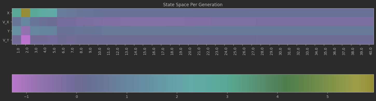
StateSpace = np.array([self.simulation.state_trajectory[T - 1].detach().numpy()])
avgSS = np.zeros([1, 4])
avgSS[0, 0] = np.mean(StateSpace[:, :, 0])
avgSS[0, 1] = np.mean(StateSpace[:, :, 1])
avgSS[0, 2] = np.mean(StateSpace[:, :, 2])
avgSS[0, 3] = np.mean(StateSpace[:, :, 3])
print(avgSS)
combAvgSS = np.append(combAvgSS, avgSS, axis=0)
plt.figure(1)
self.visualize(T, epoch)
epochNum = np.linspace(1, epochs, epochs)
plt.figure(2)
plt.plot(epochNum, lossArray)
plt.show()
# combAvgPOS=np.array([combAvgSS[:,0],combAvgSS[:,2] ])
# combAvgVel = np.array([combAvgSS[:, 1], combAvgSS[:, 3]])
#
# PosNames = ["X", "Y"]
# fig, ax = plt.subplots(figsize=(18, 10))
# im = ax.imshow(combAvgPOS)
#
# cbar = ax.figure.colorbar(im, ax=ax, cmap="YlGn", orientation="horizontal")
#
# # Show all ticks and label them with the respective list entries
# ax.set_xticks(np.arange(len(epochNum)), labels=epochNum)
# ax.set_yticks(np.arange(len(PosNames)), labels=PosNames)
#
# # Rotate the tick labels and set their alignment.
# plt.setp(ax.get_xticklabels(), rotation=90, ha="right", rotation_mode="anchor")
#
# # for i in range(len(stateNames)):
# # for j in range(len(epochNum)):
# # text = ax.text(j,i, combAvgSS.T[i, j], ha="center", va="center", color="w", fontsize="x-small")
#
# ax.set_title("State Space for Positions Per Generation")
# plt.show()
#
# velNames = [ "V_X", "V_Y"]
# fig, ax2 = plt.subplots(figsize=(18, 10))
# im = ax2.imshow(combAvgVel)
#
# cbar = ax2.figure.colorbar(im, ax=ax2, cmap="YlGn", orientation="horizontal")
#
# # Show all ticks and label them with the respective list entries
# ax2.set_xticks(np.arange(len(epochNum)), labels=epochNum)
# ax2.set_yticks(np.arange(len(velNames)), labels=velNames)
#
# # Rotate the tick labels and set their alignment.
# plt.setp(ax2.get_xticklabels(), rotation=90, ha="right", rotation_mode="anchor")
#
# # for i in range(len(stateNames)):
# # for j in range(len(epochNum)):
# # text = ax.text(j,i, combAvgSS.T[i, j], ha="center", va="center", color="w", fontsize="x-small")
#
# ax2.set_title("State Space for Velocities Per Generation")
# #plt.show()
def visualize(self, T, Epoch):
data = np.array([self.simulation.state_trajectory[i].detach().numpy() for i in range(self.simulation.T)])
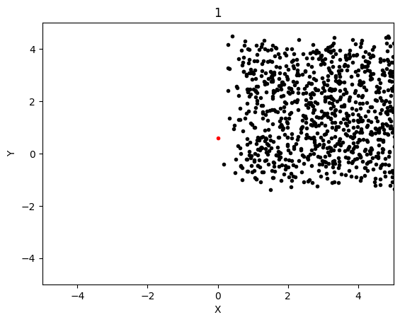
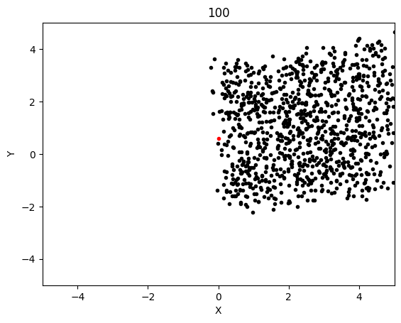
x = data[T - 1, :, 0]
vx = data[T - 1, :, 1]
y = data[T - 1, :, 2]
vy = data[T - 1, :, 3]
plt.figure(3)
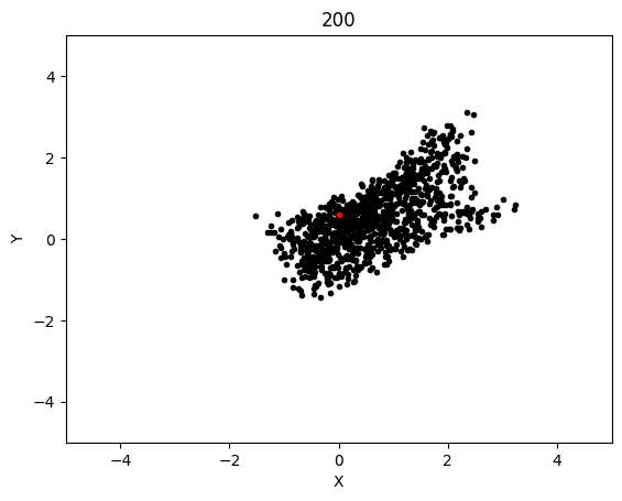
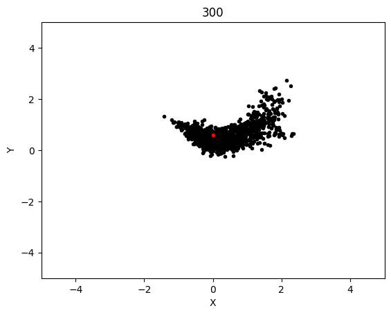
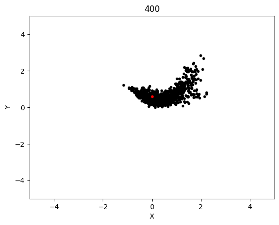
plt.plot(x, y, 'k.')
plt.xlabel('X')
plt.ylabel('Y')
plt.title(Epoch + 1)
plt.plot((PLATFORM_HEIGHT), 'r.')
plt.xlim([-5, 5])
plt.ylim([-5, 5])
plt.show()
plt.clf()
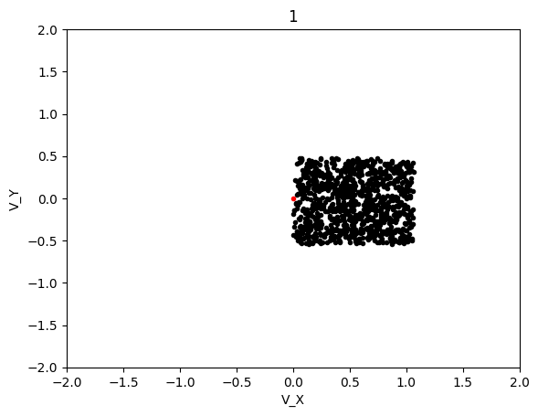
plt.figure(4)
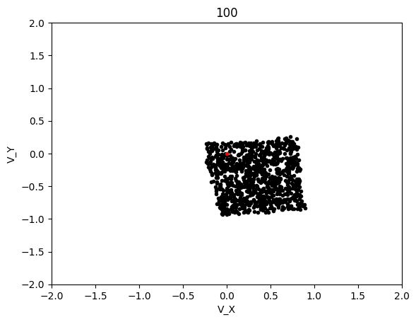
plt.plot(vx, vy, 'k.')
plt.xlabel('V_X')
plt.ylabel('V_Y')
plt.title(Epoch + 1)
plt.plot((0), 'r.')
plt.xlim([-2, 2])
plt.ylim([-2, 2])
plt.show()
plt.clf()
# Now it's time to run the code!
T = 50 # number of time steps
dim_input = 5 # state space dimensions
dim_hidden = 8 # latent dimensions
dim_h2 = 5
dim_output = 2 # action space dimensions
d = Dynamics() # define dynamics
c = Controller(dim_input, dim_hidden, dim_h2, dim_output) # define controller
s = Simulation(c, d, T) # define simulation
o = Optimize(s) # define optimizer
o.train(numOfEpochs, T) # solve the optimization problem
To solve this minimization problem we used a neural network with 2 hidden layers which took a batch of random starting states and simulated the trajectory of the rocket using given dynamics. It then attempted to control the action of the controller to minimize the loss of the simulation. This was repeated for multiple genrations and a controller was produced. LBFGS and Adamax were the two optimization programs used
See Notebook.ipynb for raw results and specific code used for this example.
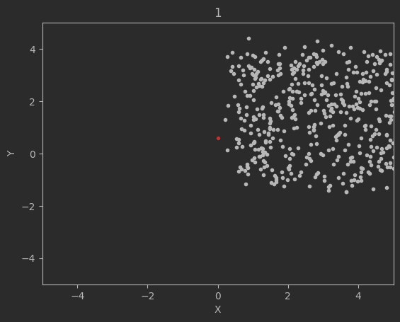
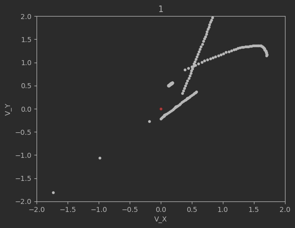
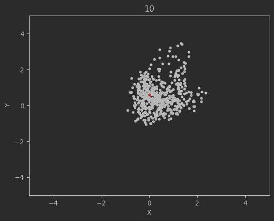
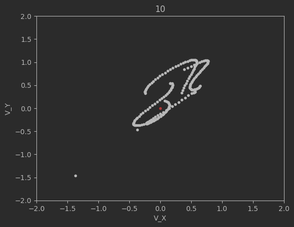
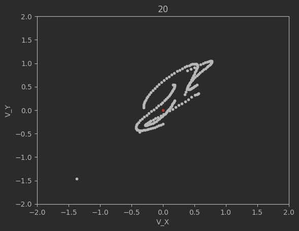
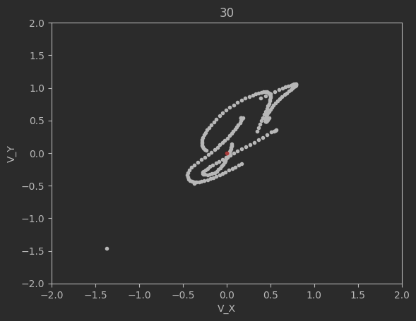
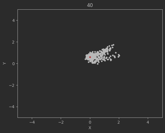
The graphs below shows the states of the rockets from each generation at T_max:
Epoch 1:
Epoch 10:
Epoch 20:

Epoch 30:

Epoch 40:

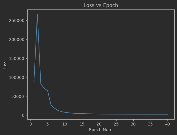
Clearly this algorithm is not perfect as seen by the spikes up in the loss and the inability of the code to significantly minimize the final velocities. Additionally, although not shown above, many times the program will fail entirely and diverge away from the target solution. There are mutliple reasons for this. The first is because of LBFGS does not use a line search, but instead uses a fixed step size. Likewise, tuning the weights and the network dimensions are difficult and lead a lot instability in the minimization.
See Adamax Optimization.ipynb for raw results and specific code used for this example.
This simulation converged significantly slower, although luckly each generation was significantly cheaper to compute so I was able to run 600 generation long test in the same time as with LBFGS. This led to the following results:
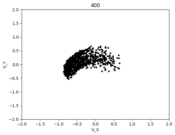
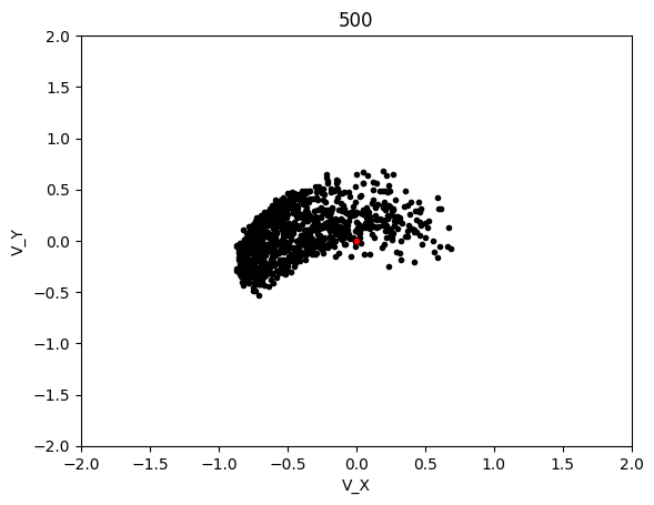
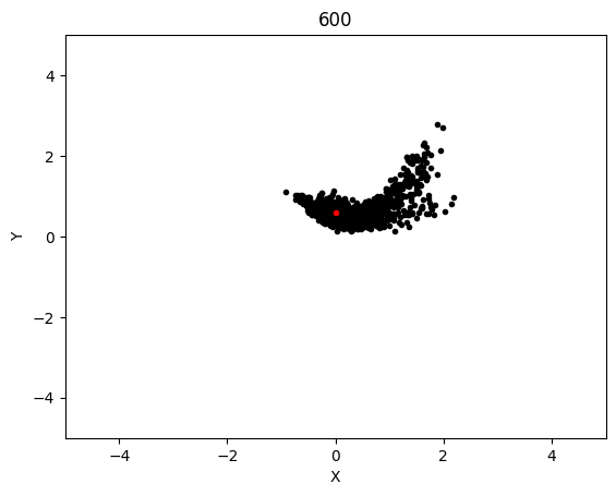
The graphs below shows the states of the rockets from each generation at T_max:
Epoch 1:
Epoch 100:
Epoch 200:

Epoch 300:

Epoch 400:
Epoch 500:

Epoch 600:

Loss Per Generation:
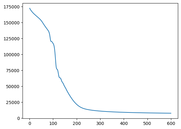
AdaMax converged significanly better than LBFGS and when running tests, it was much more likely to converge on any given test as compared to LBFGS. The rockets that failed be at the target state at T_max were probably because their initial starting state was non-recoverable, which is not covered in this project.